Time domain reflectometry: techniques and examples

Peter Herpertz - Product manager

One of the best ways of enhancing the evaluation of results produced using time domain reflectometers (TDRs) is to make comparative measurements, as comparisons invariably show the details of faults much more easily and clearly. If the equipment used has facilities for storing measurements, it is even possible to compare a single-core cable with itself, by comparing the current measurement with a stored trace. Between two measurements on the same cable, the fault can be enhanced by manipulating it – for example, by burning or by using various Arc Reflection Methods (ARM).

Typical procedure for making a reflection measurement

1. Determine the fault resistance by using an ohmmeter or an insulation tester. This insulation tester must have a measurement range of less than 1 kΩ in order to resolve resistances between 10 and 1000 Ω. Connect the reflectometer to the faulty cable and set the typical propagation velocity for the cable.
2. Select the measurement range so that the entire cable length is visible at the start of the measurement. If necessary, check on a good, fault-free core.
   Important rule:  Always ensure that the cable end is visible!
3. Where possible, set the compensation so that a horizontal trace is visible at the start of the reflectogram. The remaining small visible positive and negative deflections should be relatively symmetrical. Avoid saturation (Clipping).
4. Start the measurement with a large pulse width, and once all details including the end are recognisable, reduce the pulse width, until these details are just still visible. By doing this, the measurement will be done with the highest resolution and accuracy and will provide the highest level of detail.
5. Enhance the fault position by using the gain setting. Reduce the display range if necessary.
6. Measure the fault location. The exact measurement of the fault position is made by using the vertical cursor. Set this to the foot point of the fault reflection, which is the position where the fault reflection just starts and where it causes the first deviation from the normal horizontal behaviour of the trace. This is not necessarily a deviation from the horizontal line – it can also start within an existing reflection.
7. If possible, a comparison of good and faulty traces should be made. The deviation (splitting) of the reflectograms at the fault location, which is usually readily apparent, can be measured very easily, resulting in a high level of accuracy and easier fault recognition.

MEASURING METHODS

Direct reflection measurement line comparison

A fault-free, good core is necessary for line comparison. Alternate switching between the good and faulty lines reveals a difference between the reflectograms, which indicates the fault position.

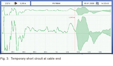
Intermittent fault location (IFL) mode

IFL Mode is intended for the localisation of intermittent faults. These are faults that appear only sporadically, in certain situations, and can usually not be reproduced in normal operation. During IFL operation, a reflectogram is continuously recorded. This records all changes irrespective of their appearance. With no fault present, the changes will only affect a small area (envelope) around the normal trace, and will only thicken it. As soon as a significant fault occurs, however, a clear change (splitting) of the envelope will be seen as shown in Fig 3 at around 1.35 km. The operator can wait for something to happen, or force the fault to change by moving or shaking the cable

Differential measurement

When the differential method is used, the good and faulty lines are connected simultaneously via a differential transformer to the reflectometer. In this mode, one line is measured in the normal way. When measuring the comparison line, the polarity of all reflections is changed by the differential transformer. This means that only real differences are shown in differential mode. Faults of the same size or completely interrupted cables cannot be seen since no difference exists.Note: When using the differential method, always ensure that the test leads are correctly connected. Interchanging the leads changes the polarity of the reflection.

Averaging

Inductive couplings or other external influences as radio stations etc. generate noise and disturbances in the trace. These disturbances can be eliminated by using the averaging mode to average multiple (up to 200 or more) measurements. 

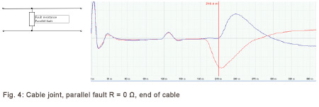
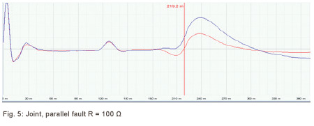
Examples of parallel faults with various resistances (negative reflection)

The closer the value of fault resistance is to the cable impedance, the less visible it becomes. When both values are identical, no reflection can be seen. This exact effect is used in the communication area for the resistive termination of circuits. (LAN, antenna circuits and other data lines). If the terminating resistor is equal to the cable impedance, no signal is reflected. The quality of a termination can be tested and verified with a reflectometer.

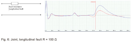
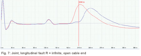
Examples of longitudinal faults with various resistances (positive reflection)
For fault location it is essential always to bear in mind that an easily visible open reflection is not necessarily the end of the cable – it can also be a break or cut in the cable. A simple test is to short the end and check if this is visible. If it is not visible, the reflection is from an interruption in the cable.

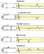
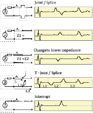
Examples of typical responses in reflection measurements

This is the final part of a five-part series by Peter Herpertz covering cable fault location. If you’ve missed either of the previous four parts, you’ll find them in the back issues of Electrical Tester, starting with the July 2013 edition. Back issues of the print edition of Electrical Tester are available online, in addition why not take a look at past issue of Electrical Tester Online too while you're here.