Instantaneous torque as a predictive maintenance tool

Authors: Leslie Reed, Technical Trainer/Application Engineer, Megger Baker Instruments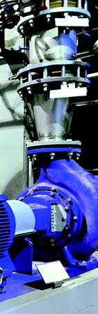

Introduction

In recent years, there have been significant advances in the on-line testing of motors, motor diagnostics and motor monitoring. Voltage and current signature analyses have greatly improved the quality of predictive maintenance (PdM) programs compared with what was possible using only measurements of RMS current and voltage or power factor.

The most advanced form of signature analysis is torque signature analysis, which provides an instantaneous torque signature derived from the current and voltage signatures. It is inherently demodulated and delivers a very clear signal independent of the line frequency (either 60 Hz, or variable in VFD applications). The instantaneous torque signature also delivers the clearest mechanical information available about the motor system, since torque production is the primary, if not sole, reason for the motor’s existence. This article looks at three case studies in which torque signature analysis has played an important role. In all three cases, measurement and analysis was performed using the Baker EXP4000 dynamic motor analyser from Megger.

BASICS OF MODERN ON-LINE MONITORING

Connectivity

On-line monitoring tools for field use must be safe and easy to use if they are to be employed regularly. A general rule of thumb in predictive maintenance says that the quality of a PdM program is proportional to the quality of the tools used multiplied by the frequency with which they are applied. In other words, only top-of-theline tools and frequent monitoring are likely to yield the most effective plant reliability program results.

Connections to medium- or high-voltage applications can be achieved safely with hook-ups to existing current transformers (CTs) and potential/voltage transformers (PTs). Unfortunately, on-line monitoring is too often performed with unsafe procedures, usually for the sake of getting a job done as quickly as possible. Responsible plant operation, however, allows only two methods for performing on-line testing safely:

• Lockout procedures using protective gear „
• Dedicated hardware in critical motor control cabinets

We’ve seen that maximising plant reliability requires frequent testing and this is unlikely to be achieved if the first method is adopted. Only the permanent installation of monitoring hardware in motor control cabinets (MCCs) will assist reliable plant operation in an easy, safe, and cost-effective manner.

Voltage quality and load level

On-line monitoring has evolved considerably from the times when state-of-the-art electrical monitoring was confined to current and voltage levels. Power quality analysers were introduced several years ago, and they are now capable of identifying and logging voltage unbalances, distortions and transients.

However, poor voltage conditions are a main cause of overheating in motors that are not overloaded [1-5], and comparisons of sub-optimal voltage quality with its effect on the motor are not possible with power analysers. Evaluation of the way that poor voltage conditions affect motors at different load levels allows maintenance professionals to ensure that the motor is running at the proper NEMA de-rating [2-4]. Only the addition of very accurate load estimations [5,7-8] to power quality analysis will offer useable results from a motor PdM standpoint.

A major concern for all motor users is whether a motor is overloaded. This can only be ascertained reliably if accurate load estimates are combined with power quality measurements and the results evaluated in line with applicable standards and guidelines [1-4].

Voltage levels and estimation errors

In the field, voltage busses are often operated at an overvoltage that exceeds 5 %. There are two reasons for this. The first is that a higher voltage on the bus can help to ensure that sufficient voltage reaches the motor terminals after subtracting the voltage drop in the connecting leads. The second reason is that over-voltage can reduce operating currents, and this is frequently considered desirable although it is usually more a case of comfort than necessity.

Stator current is known as the source of I2R losses in the motor, so increasing the voltage and reducing the current promotes a feeling of reduced losses as well as a cooler and healthier motor operation. In reality, artificially reducing the current in this way only marginally improves operational efficiency of a motor while causing severe deterioration of the operating power factor [1]. There is little effect on the operating temperature or expected life.

Artificially reduced stator currents do, however, lead to erroneous conclusions if current levels are used as a measure of load, prompting a false sense of security in the case of a motor running with an over voltage and rated stator current. In fact, motors under these conditions are operating into their service factor, which leads to overheating and rapid deterioration.

Case study #1: a 500 horsepower (HP) pulverizing machine in South Korea

Nameplate and setup

A 500 HP 6.6 kV motor was monitored in a unit of a major power generation facility in South Korea. The nameplate showed 54 A, 882 RPM as provided in Figure 1.

Figure 1: Motor nameplate information

The nameplate speed is low when compared with most eight-pole motors. Eight-pole motors of this rating have typical nameplate speeds of 885 RPM or 890 RPM. Since slip is proportional to rotor copper losses, the high slip implied by the low nameplate speed suggests that either the motor is of lower efficiency than modern designs or the nameplate is inaccurate. Testing was done in order to try and determine loading. Testing was performed using connections to the secondary terminals of the PTs and CTs. All data shown in Table 1 was obtained at the motor control cabinet (MCC).

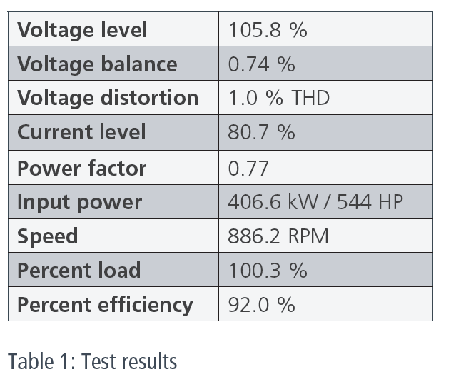
Load estimation can be done in four different ways. The first method simply divides measured current by nameplate current and multiplies the quotient by 100 %.

Figure 2: Slip line and operating point

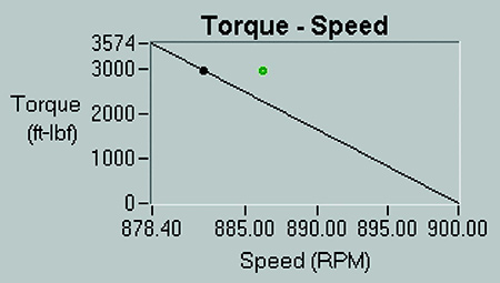
Figure 3: Instantaneous torque

For this motor, the resultant load estimation is 80.7 % (note that with a 0.77 PF, the load would have to be less than 80.7 %). These results show how misleading it can be to only focus on RMS values. By using the current alone as an indicator of the load on the motor, it would be reasonable to say that the loading was less than 80 %. The actual load of 100.3 % is, however, much higher than the calculation based on current suggests.

The second method of loading assessment is based on slip. By using the nameplate data, the load would be estimated at 76.7 %. This figure is obtained by dividing the actual operating slip by the rated slip.

[(900-886.2)/(900-882)]*100 = 76.7 %

When the motor was monitored, it was found to have much lower slip than suggested by the nameplate slip line, as indicated in Figure 2. The black line is the slip line based on nameplate information. It runs from the synchronous point at the lower right, where the speed is 900 RPM and the torque is zero, to the rated point, which is shown by the black dot. The actual operating point is shown by the green dot to the right of the line. This reveals that the motor is running at a higher speed than the nameplate would lead one to expect.

The third method for load estimation uses input power. Input power is calculated by multiplying voltage, current, power factor, and square root of 3. The calculation indicates that the input power for this motor is 544 HP, or 8.8 % more power going to the motor than its rated output of 500 HP. This poses the question: is the motor running at an overload with a very high efficiency or is it running at 100 % load with a very low efficiency? Standard instrumentation cannot answer this question.

The fourth method combines the speed method with torque. The mechanical output power of a motor is calculated by multiplying the shaft torque by the operating speed. Operational torque is calculated using Park’s vector, which is also called the two-axis theory [6-8]. The rotor speed is calculated using current signature analysis [5, 7-8]. Dividing the mechanical output power by the electrical input power gives the operational efficiency. As already noted, none of the three conventional approaches – speed-based load estimation, stator current load estimation or input power estimation – can give clear information about the loading and operating efficiency of the motor.

To truly operate a motor at 100 % load, it is necessary to have a very good power quality. In the present application, this requirement is met because the voltage imbalance is small (i.e. less than 2 %) and there is low voltage distortion. The voltage is notably high, but not high enough to cause concern.

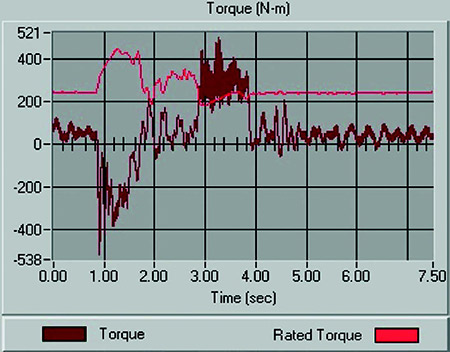
This application involved a motor driving a coalpulverising machine, and machines of this type are notorious for abrupt changes in torque, depending on the size of the pieces fed into them. Figure 3 shows the instantaneous torque plotted against the machine’s rated torque.

The rated torque is calculated from the nameplate speed and horsepower. The brown trace shows the actual instantaneous torque calculated according to E. Wiedenbrug and others [5]. It is clear the average torque coincides with the rated torque which is to be expected with the load at 100.3 %. However, the torque ripple added to the steady-state torque causes the motor to operate from time to time under ‘over-torque’ conditions (greater than 115 % of the rated torque). In other words, the motor is operating above its rated load for significant periods of time.

This is a typical marginal application that stresses the motor. A reduction in the amount of coal fed into the pulverising machine will reduce the motor load to a healthy operational level.

Case study #2: detection of mechanical problem saves millions of US dollars

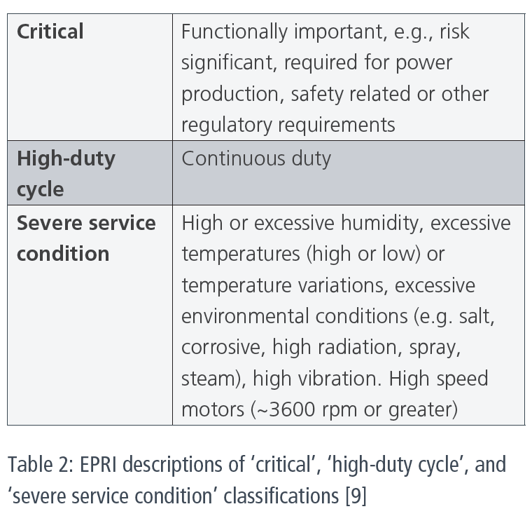
This case study is based on data obtained from tests conducted at a coal-fired power plant in the USA. The motor under consideration falls into the category of “critical, high-duty cycle and severe service condition” according to EPRI [9] (Table 2).

Motor application

The motor was one of three circulating water pumps at a power generation plant with a total output power of 732 MW. The plant’s total output is nearly proportional to the combined output of the pumps. All three pumps fed into a single system, which had just one total flow meter. There were no independent flow meters to monitor the individual pumps. The motors driving the other two pumps were operating at slightly slower speeds with higher stator currents. Since the load was underwater (a deep submerged pump) it was impossible to conduct vibration monitoring.

The difference between the speed and operating current of the motor under consideration and the other two raised concerns, but no conclusive evidence of malfunctioning was obtained by using standard motor test instrumentation. Because of this lack of evidence, the critical nature of the application and the need for continuous operation, maintenance personnel decided not to stop the pump for further investigation.

Figure 4: Torque signature of a healthy circulating pump

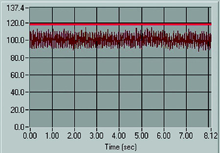
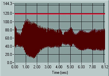
Figure 5: Torque signature of the pump causing concern

However, when a modern on-line monitoring instrument was connected to the pump motor, this provided instantaneous torque measurements that ultimately led to identification and diagnosis of a problem.

Results

Results from the on-line instrument confirmed some expectations. The third motor was indeed requesting less input power, leading to lower power factor and lower stator current linked to higher operating speed. What was more interesting was a comparison of the instantaneous torque signatures from the motor causing concern and the other two motors. Figure 4 shows the instantaneous torque of a healthy pump.

The full red line is the rated torque line. As can be seen, this pump operates at a high average torque level, but safely below the full rating. The torque ripple is small and constant. This signature is typical of a pump without flow regulation.

The torque signature of the pump causing concern (Figure 5) differs considerably from the signature of the healthy pump. One of the main differences is that that the steady-state torque is about 75 % of that of the healthy pumps, which are working in a nominally identical application. Further, the torque ripple is not typical for a healthy large pump. The torque band is too wide, and it does not have a steady envelope.

Since the motor must deliver the torque requested by the load, it was possible to state without any doubts that this pump had severe problems. Prior to this, it had not been clear whether it was the pump or the motor that had problems. The information provided by the torque signature analysis justified stopping the pump and sending a diver to examine it. The diver quickly discovered that the pump had lost its end bell. Figures 6 and 7 show the pump and the end bell.

Figure 6: Pump

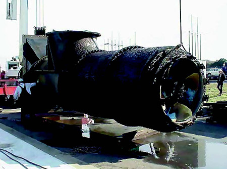
The function of the end bell is similar to that of a funnel: it aids laminar flow of water into the pump. Without the end bell, the impeller of the pump is in close to the opening of the pump, which means that the slow-turning impeller only partially works as a pump. Water circulates within the pump instead of down the pipe, which explains why the torque is so low (it takes less power to keep water circulating within the pump than it takes to pump the water). Additionally, when the blades are close to standing water, they create turbulence and cavitation. This was the source of the additional torque ripple that had been found during on-line testing.

Repair

Upon discovery of the broken end bell, the pump was pulled for repair. After repair, the pump was immediately placed back in operation, and subsequent on-line testing revealed that the torque level was back to a normal, higher range. The torque ripple of this pump and the other two decreased noticeably compared with previous results. The plant’s maintenance personnel concluded that the pressure fluctuations caused by the cavitation might have propagated through the piping and slightly influenced the two healthy pumps, adding to their torque ripple.

Ramifications to a related failure

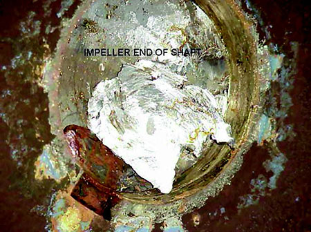
One week after the pump was repaired, one of the two adjacent pumps broke a shaft. Figure 8 shows the broken shaft at the impeller end. This failure had to be repaired immediately; removing the pump from operation, repairing, reconditioning and re-installing took five weeks. The plant maintenance personnel concluded that this failure could have been linked to the additional torque ripple created by the broken end bell of the first pump. To date, it has been impossible to prove or disprove this suggestion.

Figure 7: End bell

Figure 8: Broken shaft at impeller end

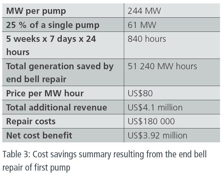
Cost savings

During the five weeks it took to remove, repair and reinstall the second pump, the power plant had to operate at reduced capacity. However, the pump with the repaired end bell was able to deliver 25 % more output than at pre-repair levels and this helped to offset the losses. This additional output would not have been available without the evidence provided by the instantaneous torque signature which demonstrated conclusively that the repair was needed.

A calculation of additional output power available as a result of the end bell repair was performed. This was based on the plant’s rating of 732 MW, and the assumption that this power is attained when all three pumps are in full operation. Table 3 summarises calculations of the cost savings that resulted directly from the detection of the end bell problem.

Case study #3: a conveyor problem solved

This case study concerns a variable frequency drive (VFD) application for a conveyor system at a pulp and paper mill in Canada. A 60 HP, 1170 RPM 460 V motor driving a conveyor belt is controlled by a variable frequency drive (VFD). The conveyor belt feeds logs into a saw. When no log is in the saw, the conveyor belt runs at high speed; when a log approaches the saw blade, the conveyor belt slows down to a speed optimised for cutting. Shortly after it detects that the log has left the saw, the conveyor returns to high speed.

Figure 9 graphically depicts the process showing frequency (red) and voltage (blue) versus time. Data was captured over a period of 7.5 seconds. The VFD runs the motor at 60 Hz, and then slows it down to 12 Hz for cutting. Cutting a log takes less than 1.4 seconds after which the VFD ramps the frequency back up to 60 Hz.

This VFD uses V/f control where the voltage is proportional to the operating frequency. This type of control is very common in low cost implementations.

Figure 10 shows torque (red) and the operational speed (blue) of the motor versus time. It reveals that the maximum speed of the motor is 1200 RPM, but the speed of the motor while cutting a log is only 215 RPM.

Figure 9: VFD frequency and voltage level vs. time

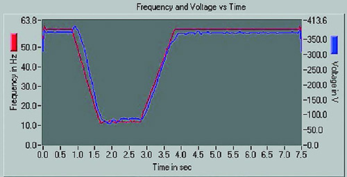
Figure 10: Speed and torque vs. time

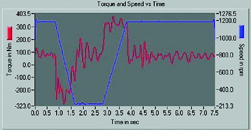
Torque level is constant when the conveyor operates at constant speed. When the VFD backs the voltage down, the motor speed slows in response to the reduced torque. As soon as the low speed is reached, the torque level stabilises at the steady-state level.

During the subsequent acceleration process, the torque level increases before falling back to the steady-state level when acceleration is complete.

During deceleration, the torque at first drops rapidly. It even drops below the zero-torque line, which means that the motor is acting as an electrical brake. It also means that the log slows down rapidly as the motor speed reduces by around 1000 RPM in just one second. This information is important because it means that the conveyor has to be designed not only for pulling, but also for pushing.

Figure 11 shows the torque versus time curve in more detail and it is noteworthy that over a period of about one second, the operational torque rises above the rated torque. This means the motor is stressed during acceleration. The torque required to accelerate the log to 1200 RPM back from 215 RPM is too high, especially if this has to be done in less than one second.

The solution to this dynamic over-torque problem is simple. The VFD has a programmable Hz/sec setting which limits the maximum acceleration and deceleration rates. In this case, the maximum acceleration rate was too high but reducing the Hz/sec setting brought the acceleration torque down to an acceptable level. A disadvantage is that acceleration and deceleration times are increased which might lead to reduced throughput. In this case, however, the change in settings increased the acceleration and deceleration times by just 0.2 sec, which had no noticeable effect on productivity.

Another issue was identified by inspecting the last three seconds of data. The operational torque over this period is oscillating, which is a typical symptom of an improperly tuned feedback loop. The application is ‘chasing,’ and is unable to maintain a steady state speed free of oscillations. This oscillation fatigues the conveyor system and could lead to premature wear and failure. It can be avoided by installing a properly tuned PID controller, but it needed the torque signature analysis to show that this would be beneficial.

Figure 11: Instantaneous torque vs. time

In this application, the three issues revealed by the analysis of the torque signature have straightforward solutions, but they couldn’t have been identified with standard motor test and monitoring instrumentation. Only instrumentation that is capable of displaying the dynamics of a VFD application can uncover problems of this type, thereby providing the information needed to ensure that systems operate reliably.

Conclusion

Case studies like those in this article demonstrate why more companies are adopting predictive maintenance programs based on on-line monitoring of motors. The first scenario illustrated how it is possible to identify loadings that will lead to rapid motor deterioration and showed that load estimation based on input power, input current or operating speed is unreliable. The second scenario showed how reliable load diagnostics can help with rapid problem identification and diagnosis, ultimately leading to big cost benefits, while the third showed that the load diagnostic techniques are equally useful in the growing number of motor applications that use VFDs.

Finally, this article stresses that on-line electrical monitoring and analysis is necessary to maximise plant reliability. It would not have been possible to diagnose any of the three cases presented here without using online tools capable of displaying instantaneous torque.

REFERENCES

[1] Ongoing issues with electric motors – Austin Bonnett, Na tional Motors and Drives Steering Committee, Montreal, June 2000.

[2] NEMA MG1, Part 14, 1998.

[3] Voltage Unbalance: Power Quality Issues, Related Standards and Mitigation Techniques, EPRI Technical Report – A. van Jouanne.

[4] NEMA MG1, Section IV Part 30 1998.

[5] Modern on-line testing of Induction Motors for Predictive Maintenance and Monitoring – E. Wiedenbrug, Ph.D., A. Ramme, E. Matheson, A. van Jouanne, Ph.D., A. Wallace, Ph.D. IEEE IAS Pulp and Paper Conference 2001, Portland, OR, USA.

[6] Analysis of Electric Machinery – Paul C. Krause, et.al. IEEE Press, New York, 1995.

[7] Measurement Analysis and Efficiency Estimation of Three Phase Induction Machines Using Instantaneous Electrical Quantities – E. Wiedenbrug, A dissertation submitted to Oregon State University September 24th, 1998.

[8] In-service Testing of Three Phase Induction Machines – E. Wiedenbrug, A. Wallace, SDEMPED IEEE Gijon, Spain 1999.

[9] Preventive Maintenance Basis, Volume 10: High Voltage Electric Motors (5 kV and greater), Final Report, July 1997 EPRI, Prepared by Applied Resource Management 313 Nobles Lane.