Testing power swing and out-of-step relay elements using simplified equations

The method

Past methods of testing power swing and out-of-step conditions have often involved a brute force approach of applying voltages and currents to simulate impedances seen by the relay. By manually ramping the impedance trajectory, or playing several vector states where specific impedance was applied, it was possible to trick the relay into seeing an impedance tracking across the measurement zones. However, trying to trick new relays with more advanced algorithms doesn’t work. The relay is looking for a smooth transition between the measurement zones, and if it does not see it, then it will not block the power swing or trip on the out-of-step.

To satisfy the conditions for the power swing and out-of-step algorithms currently in use, a new method is proposed. By superimposing two waveforms of similar frequencies, a smooth impedance ramp can be achieved. This method is similar to a two-source model in that both sources have similar frequencies and amplitudes. The rate of change of impedance can be controlled as well as the minimum and maximum impedances, the number of pole slips, and the starting phase angle relationships. The characteristic equation of the output waveform for the voltage and current is as follows:

Eq. 1   f(I,V) (t)=(A1  sin(ω1 t+φ1 ) )+A2  sin(ω2 t+φ2 ) 

Where:
A1 = Magnitude of current/voltage source 1 as an RMS value
ω1 = 2π*FrequencySource1 , (Frequency is in Hz, ω1 is in rad/s)
φ1 = Initial phase angle of current/voltage source 1 in degrees
A2 = Magnitude of current/voltage source 2 as an RMS value
ω2 = 2π*FrequencySource2 , (Frequency is in Hz, ω2 is in rad/s)
φ2 = Initial phase angle of current/voltage source 2 in degrees
t = the time of the event in seconds

Using arbitrary values for Equation 1, Figure 1 shows the plot of a voltage and current waveform with the following parameters:

V1= 49.5 V,   V2=19.5 V,   I1=16.725A,   I2=13.275A,   F1=60 Hz,   F2 = 59 Hz,

φ1Current = 0°,   φ2Current = 0°,   φ1Voltage = 0°,   φ2Voltage = 0°

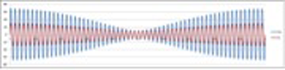
Figure 1 – Superimposed voltage and current waveforms

Both the voltage and current waveforms decrease and increase at the same time and remain in phase for the duration of the waveform plot. This is not the behaviour of a power swing or out-of-step condition. To change this, the phase current needs to be offset by 180°. The option is to change either φ1Current or φ2Current. By changing φ1Current, the phase angle will initially start 180° out of phase and then slowly come back into phase, then go back out, and repeat indefinitely. Since it is desirable to control the phase angle from the start, φ2Current will be set to 180°. This will allow the two waveforms to start in phase and then slowly go out of phase and come back into phase, and repeat. A plot of the waveforms with the appropriate phase shift is shown in Figure 2.

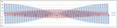
Figure 2 Plot of voltage and current waveforms with current offset by 180°

This is the general form of the power swing waveform. Next is a discussion on how to implement a controlled power swing and out-of-step condition using any of the Megger SMRT test systems.

Applying the method

Power Swing

To apply a power swing, the following parameters need to be defined.
  

1. The Maximum Impedance, Zmax, of the Power Swing/Out-of-Step needs to be defined. This will be based on the outermost characteristic that is tracking the impedance. It is recommended that the maximum impedance be greater than the largest blinder/characteristic impedance, but not so large that the trajectory of the swing exits the characteristic prematurely.
2. The Minimum Impedance, Zmin, of the Power Swing/Out-of-Step also needs to be defined. This will be the stopping point of the swing/step.
3. The Source Frequencies will determine the duration of a single power swing or out-of-step condition. The source frequencies will also affect the rate of change of the trajectory of the impedance. The larger the difference in frequency between the two sources, the faster the swing/step, and the smaller the difference, the slower the swing/step.
4. The Starting Phase Angle needs to be defined so that proper loading conditions can be simulated.

Here is how to create a power swing with a maximum impedance of 15 Ω, a minimum impedance of 1 Ω, a Source 1 Frequency of 60 Hz, a Source 2 Frequency of 59 Hz, and a starting Phase Angle of 0°.

The first parameter that we can determine is how long a complete power swing cycle will take, tSwing.  This is given by Equation 2.

Eq. 2   tSwing=1/(f1-f2 )  (s)

Putting our values into this equation:

tSwing=1/(60-59)=1 s

When applying this method to any type of test routine, tSwing should be set for the maximum time the swing should be applied. If multiple turns are desired, then maximum time is the number of turns times tSwing. 

Next, we will be solving for the currents and voltages that should be applied to the relay. To start, only the A phase voltage and current will be discussed. B and C phases are identical to A, with the appropriate phase shifts. A nominal voltage should be defined for the maximum impedance, and a fault voltage should be defined for the minimum impedance. Take care in choosing a fault voltage. Some of the impedances could still be quite large, with large being defined as around 15 Ω or greater. If the fault voltage is too small, negative currents will be calculated to create the correct conditions. If this happens, increase the fault voltage until the currents are at an acceptable level. For this example the nominal voltage, Vnom, is 69 V line-to-ground, and the fault voltage, Vfault, is around 30 V line-to-ground. 

The value of Vfault can change depending on the impedance and the current required from the test system. The variable name Vfault can also be a little misleading. A power swing event may not necessarily involve the extreme values of traditional fault voltages. The impedance swing may only go from a large value to a slightly smaller value. This would be the case if the user wanted to swing from 89Ω to 50 Ω. The required fault voltage would not be much less than that required for starting impedance.

The equations for the two voltages for phase A are:

Eq. 3   V1=Vfault+((Vnom-Vfault)/2)

Putting our values into this equation: V1=30+((69-30)/2)=49.5 V

Eq. 4   V2=((Vnom-Vfault)/2)

Putting our values into this equation: V2=((69-30)/2)=19.5 V

Then the two currents for I1 and I2 will be solved.

Eq. 5   I1=[(Vfault/Zmin )-(((Vfault/Zmin )-(Vnom/Zmax ))/2)]

Using our values:

I1=[(69/1)-(((30/1)-(69/15))/2)]=17.3 A

Eq. 6   I2=(((Vfault/Zmin )-(Vnom/Zmax ))/2)

Using our values:

I2=(((69/1)-(69/15))/2)=12.7 A

Other parameters can now be solved such as the rate of change of impedance.  Since the swing goes from maximum impedance to a minimum and back again, the rate should only be calculated based on the time it takes to go from the maximum to the minimum.  This is shown in Equation 7.

Eq. 7   Zrate=2*((Zmax-Zmin)/tSwing )

Using our values:

Zrate=2*((15-1)/1)=28 Ω/s

When starting in the pre-fault mode for testing, it is handy to be at the same current level as the starting current for the swing. This is minimum current, which is given by Equation 8.

Eq. 8   Imin=I1-I2

Using our values: 

Imin=17.3-12.7=4.6 A

For practical applications, three states can be used to simulate a pre-fault, fault and post-fault state. Figure 3 shows recorded waveforms from the Megger SMRT relay test system.

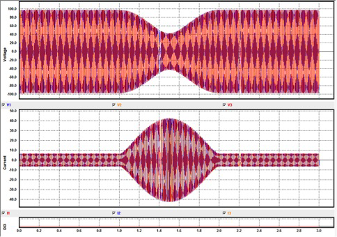
Figure 3 – Waveform capture of a power swing

The time set for the Pre-Fault duration is critical in that it is necessary for the waveform to end at the precise phase angle and magnitude that is equal to the start of the power swing event. The Pre-Fault phase angle of the current should be equal to the starting phase angle of the power swing. In Figure 3, the duration was set for 1 second, and the calculated time of 1 power swing was also 1 second. By setting the Pre-Fault to the same time as the calculated time of the power swing, a smooth transition is guaranteed in the waveforms. The time can also be set to an integer multiple of the swing duration. In this case, 2, 3, or 4 seconds would also work. A time of 0.5 seconds would not work.  This is shown in Figure 4.

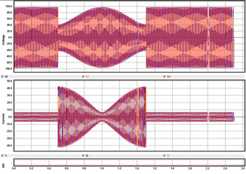
Figure 4 – Power Swing with Pre-Fault Duration changed to 0.5 s

Comparing Figure 3 and Figure 4, the shift of the power swing characteristic is apparent when the Pre-Fault duration is changed to a value other than an integer multiple of the time of the swing event. The Pre-Fault duration, or any state before a swing event should be set according to Equation 9.

Eq. 9  Tprefault=N*tSwing 

Where N is an integer (whole number)

It should be noted that if it is desirable to have flexible Pre-Fault times, the initial current and voltage magnitudes can be solved for using Eq. 1 for the applied times.

While testing the power swing element, other parameters should be displayed as well. The user will be interested to see the impedance trajectory of the power swing. This should be plotted in the R-X plane so the user can trace the circular path. The instantaneous impedance, Z, is calculated, followed by the phase angle, θ. The instantaneous impedance, Z, is defined by Equation 10.

Eq. 10    Z=V/I

The phase angle, θ, is defined in Equation 11.

Eq. 11    θ=(tVzero-tIzero )/(1/(f*360))

Where:
tVzero = time of the voltage magnitude zero crossing in seconds
tIzero = time of the current magnitude zero crossing in seconds
f = frequency of the waveform in Hz

The phase angle of power swing is shown in Figure 5.

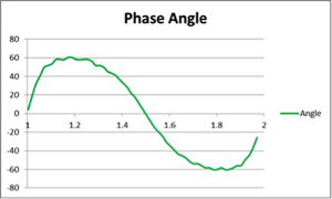Figure 5 – Phase angle of the power swing in degrees vs time in seconds

The frequency of two superimposed waveforms will not be constant. Signal processing techniques should be used to make an accurate measurement of the frequency as well as the phase angle. Equation 11 is given as a reference and will not provide a very accurate phase angle unless a very large sampling rate is used to determine the zero crossing of the waveform.

Once the impedance and phase angle are known, the resistance, R, and reactance, X, of the impedance can be determined as shown in Equations 12 and 13 respectively.

Eq. 12    R=Z*cosθ

Eq. 13    X=Z*sinθ

Once the resistance and reactance are determined, they can be plotted. This is shown in Figure 6.

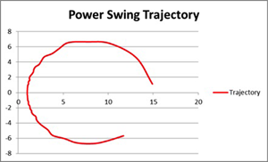
Figure 6 – Trajectory of impedance during a power swing

The trajectory starts out at the maximum impedance of 15 Ω and travels in an arc towards the minimum impedance of 1 Ω, and then circles back towards 15 Ω. The process will repeat if the swing is unstable. To simulate an unstable swing, simply increase the duration of the swing in integer multiples.

Out-of-Step

Applying an out-of-step condition is very similar to applying a power swing condition. The only difference is that instead of the impedance turning around when the minimum impedance trajectory is reached, the trajectory will continue through the origin and exit out of the other side of the characteristic. In order to achieve this a few things need to be done.

The total time of the out of step condition will be the same as the total time for a power swing, tSwing. However, changes need to be made at the halfway point of the total time in order to create an out-of-step. This time is important, so it will be called, tevent, and is equal to ½ the time of tSwing as shown in Eq. 14.

Eq. 14    tevent=tSwing/2

At time tevent, the frequency and phase angles of currents I1 and I2 need to be swapped. This will create a waveform that will continue to a phase angle difference between the voltage and current of 180°. All other calculations are the same. 

The waveforms in Figure 7 are very similar to that of Figure 3, but convey two totally different things. The difference is in the phase angle relationship between the voltage and current. Where the power swing would have a maximum phase angle difference of 90°, the out-of-step condition has a maximum phase angle difference of 180°. The phase angle relationship over time is shown in Figure 8.

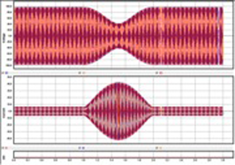
Figure 7 – Waveform capture of an out-of-step condition

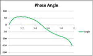
Figure 8 – Phase angle relationship of the out-of-step condition vs time

The impedance trajectory is also split. Instead of the circular path of the power swing, the return portion of the trajectory is flipped 180° so that it continues to the other side of where the relay characteristics would be located. This is shown in Figure 9.

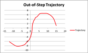
Figure 9 – Impedance trajectory of out-of-step condition

Based on the analysis given in this article, it can be seen that it is possible to implement power swing and out-of-step scenarios using simplified algebraic equations.